Learn Know-how
What are transfer functions? – Frequency Characteristics of Transfer Functions
2016.10.20
Points of this article
・An example was given in which a transfer function represents ΔVout as the result of impedance division of ΔVin by a capacitance and a resistance.
・The term 1/
・Bode diagrams (frequency characteristics) are essential. Gain and phase must be conceptualized and understood properly.
Frequency characteristics of transfer functions
Here we consider transfer functions from the standpoint of “Frequency Characteristics of transfer functions”. The explanations of “Kirchhoff’s Laws and Impedance” in the previous section are closely related, and so should be read in conjunction with this section.
First, consider Fig. 6. This is a simple closed circuit consisting of a resistor and a capacitor. We begin by determining the transfer function for this circuit.
In order to aid visualization, the circuit diagram of Fig. 6 is rewritten as in Fig. 7. Of course, the two circuits are the same. From Fig. 7 we immediately see that ΔVout is the result of dividing ΔVin by the impedances of R and C.
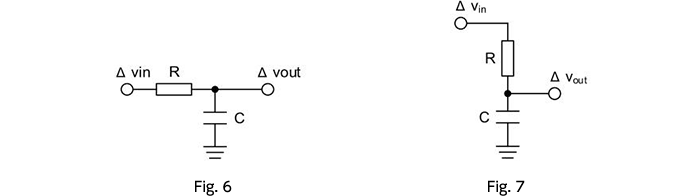
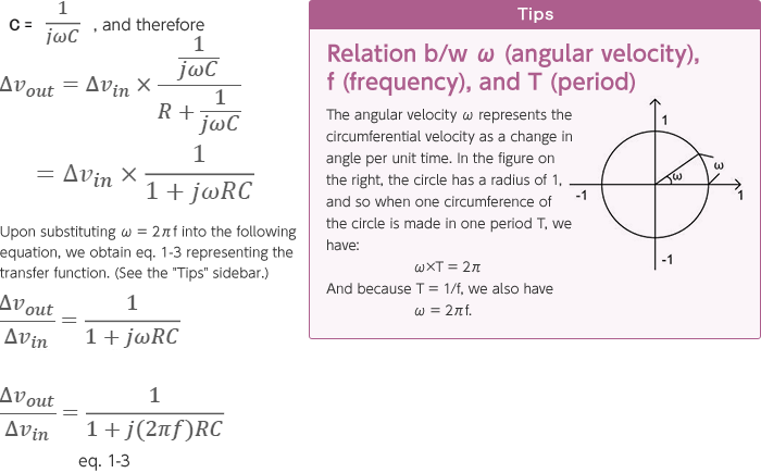
Expressed as an equation, this is ΔVout = ΔVin × (C/R+C)), but we use an impedance representation. As explained in the previous section on “Kirchhoff’s Laws and Impedance”, the impedance of R is represented by R, but for C we have
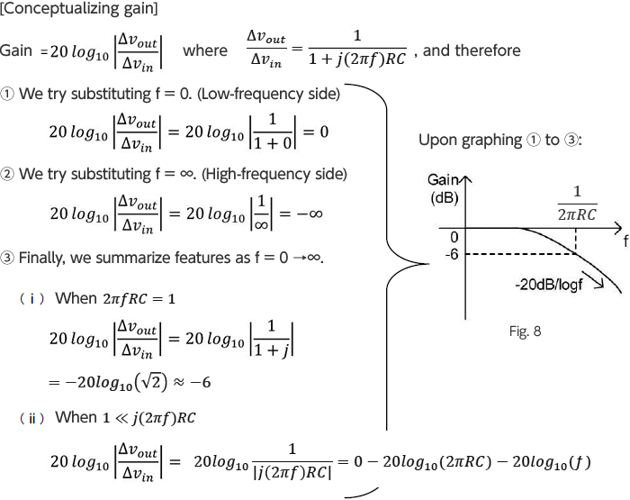
Next, we try drawing a Bode diagram. A Bode diagram represents the frequency (f) along the horizontal axis and the gain and phase along the vertical axis, and so the gain and phase must be determined. We begin by finding the gain.
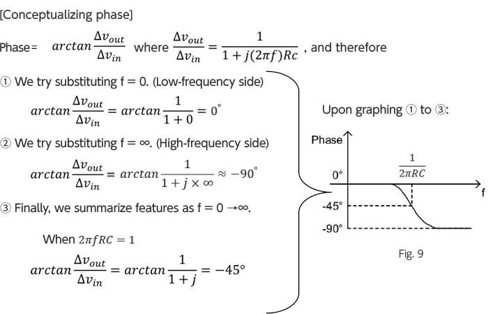
Next, we determine the phase.
The above is summarized in Fig. 10 below. From this the behavior of the gain and phase characteristics should be clear.
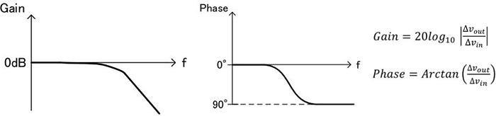
Fig. 10
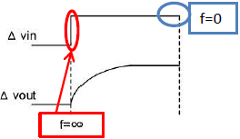
Fig. 11
In the previous section on “Kirchhoff’s Laws and Impedance”, it was stated that the impedance of a capacitor is written “1/
Fig. 11 illustrates the step response characteristic of the circuit of Fig. 6. At the moment of a fluctuation in the power supply (equivalent to f = ∞), the capacitor impedance becomes zero, and ΔVout = 0. After a certain time has passed (equivalent to f = 0), it becomes equal to ΔVin.
This can be illustrated as follows, describing the impedance 1/
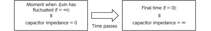
Fig. 12
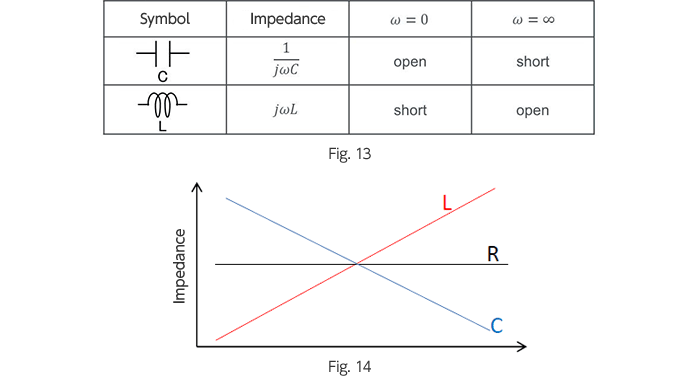
Finally, Fig. 13 gives the impedance representations for elements including a coil as well, and the circuit equivalents for the components when ω = 0 and when ω = ∞, while Fig. 14 describes their frequency characteristics.
Learn Know-how
Opamps
Transfer Function
- What are transfer functions?
- What is the Transfer Function of an Amplifier?
- What is the Transfer Function of a Slope?
- What is the switching transfer function?
-
Transfer function of each converter
- Example of Derivation for a Step-Down Converter
- Example of Deviation for a Step-up Converter
- Example of Derivation for a Step-Up/Step-Down Converter – 1
- Example of Derivation for a Step-Up/Step-Down Converter – 2
- Switching Transfer Functions: Derivation of Step-down Mode Transfer Functions Serving as a Foundation