What is Impedance? AC Circuit Analysis and Design

table of contents

• ・Basic Impedance Concepts and Complex Representations
• ・Impedance and Frequency
• ・Impedance Combination Rules and Calculation Methods
• ・Impedance Matching and Transmission Lines
• ・Impedance Measurement Methods and Troubleshooting
• ・Impedance Summary

Electrical impedance is a measure of how much an AC circuit opposes the flow of electric current. While resistance has a value that does not depend on frequency, impedance is strongly frequency dependent. This is because impedance includes not only the resistive component, but also the reactance produced by inductors and capacitors.

As a familiar example, consider the combination of headphones and an audio amplifier. The overall sound quality, frequency response, and achievable sound pressure level are influenced not only by the driver characteristics and amplifier distortion, but also by the relationship between the input and output impedances of the two devices. In this article, we cover the fundamentals of impedance and show how to apply them, ranging from familiar everyday examples to semiconductor circuit design.

Basic Impedance Concepts and Complex Representations

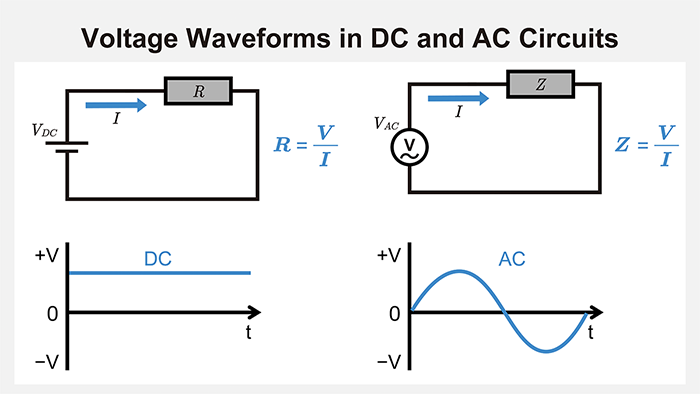
In an AC circuit, impedance is defined as the ratio of the voltage across a circuit element to the current flowing through that element. The critical point here is that, unlike a simple resistance, impedance has frequency-dependent characteristics.

A resistor dissipates energy as heat. Inductors and capacitors, by contrast, store and release energy each AC cycle, and this energy exchange appears as reactance. This is why impedance is strongly frequency‑dependent. When a datasheet specifies an impedance value in ohms (Ω), it represents the overall opposition to AC current flow at the stated frequency.

Impedance Definition, Basic Formula (Z=V/I), and the Meaning of the Ohm Unit

Impedance is defined as:

\(Z=\displaystyle\frac{V}{I}\)

It uses the same unit as resistance: the ohm (Ω). This illustrates the fundamental relationship between voltage and current in an AC circuit. Impedance Z is obtained by dividing the voltage V across a circuit element by the current I flowing through that element. In sinusoidal steady state, we typically analyze AC circuits using phasors (complex RMS quantities). Under this convention, V and I are complex values and Z is generally a complex quantity, so the relationship V = ZI has the same form as Ohm’s law.

The Impedance of the basic circuit elements are:

\(Z_R=R,　Z_L=jωL,　Z_C=\displaystyle\frac{1}{jωC}=-j\displaystyle\frac{1}{ωC}\)

Here, j is the imaginary unit and satisfies j²=-1. In AC circuit analysis, impedance is written as a complex number so that we can handle phase shifts of ±90° between voltage and current generated by inductors and capacitors. The symbol j is used to indicate the imaginary part.

The quantity ω is called the angular frequency. It is related to the ordinary frequency f in hertz by

\(ω=2πf\)

Because voltage and current vary with time in AC, simple real numbers are not sufficient. We express impedance as a complex quantity that contains both magnitude and phase information.

Relationship between Resistance R and Reactance Component X (Complex Impedance Fundamentals)

Impedance consists of two components: resistance R and reactance X. Resistance represents the dissipative part of impedance (energy loss as heat), while reactance represents the energy-storage part (inductors and capacitors). In contrast, reactance is a frequency-dependent component that arises from inductors and capacitors, modifying the overall impedance of the circuit. This is why filters, resonant networks, and EMI/signal-conditioning circuits behave differently across frequency.

Complex Impedance, magnitude, and phase angle

Complex impedance is written as

\(Z=R+jX\)

where the real part R is the resistive component and the imaginary part X is the reactance. The imaginary unit “j” facilitates the distinction between the real and imaginary parts.

When we want to treat impedance similarly to a resistance value, we usually refer to its magnitude (absolute value)

\(|Z|=\sqrt{(R^2+X^2)}\)

The phase angle θ of impedance is given by

\(θ={tan}^{-1}\left(\displaystyle\frac{X}{R}\right)\)

In this sign convention, the inductive reactance X_L and capacitive reactance X_C are both treated as positive magnitudes. On the complex plane, the inductor appears as +jX_L and the capacitor as –jX_C. When their magnitudes are equal, the imaginary parts cancel each other out.

These relationships allow us to understand circuit behavior both numerically and visually.

Impedance and Frequency

Impedance changes with frequency. Resistance is independent of frequency, but an inductor makes current flow more difficult as frequency increases, while a capacitor makes current flow easier at higher frequencies. Understanding this difference is essential for accurate circuit design.

Resistance and frequency (why resistance is frequency independent)

In DC circuits, voltage and current remain constant over time, whereas in AC circuits, they vary sinusoidally. For example, we can write instantaneous values of AC voltage and current as

\(v(t)=V sin⁡(ωt)\)

\(i(t)=I sin⁡(ωt)\)

where ω=2πf is the angular frequency corresponding to frequency f.

In a circuit that contains only resistance, the peaks and valleys of the voltage and current waveforms occur at the same time. There is no phase difference between them, so the same Ohm’s law as in DC applies. Because the instantaneous values keep changing, it is more convenient to use effective (RMS) values. If the RMS voltage is V_rms and the resistance is R, the average power is

\(P=\displaystyle\frac{V_{rms}^2}{R}\)

This is true for both DC and AC as long as the RMS voltage is the same. In other words, ideal resistance has a constant value, R, that does not depend on frequency; therefore, the relationship between voltage, current, and power remains unchanged even as the frequency varies.

In real components, very high frequencies can introduce effects such as skin effect and parasitic inductance and capacitance, resulting in slight changes to the effective resistance and phase angle. In practice, you can check the frequency characteristics and self-resonant frequency in the component datasheet.

Temperature effects on resistance and Joule’s law

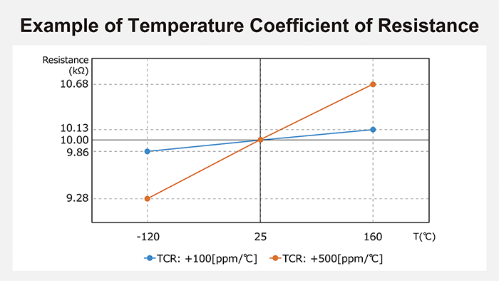
Resistance is independent of frequency, but it is affected by temperature. Many materials have a temperature coefficient, meaning their resistance value changes with changes in ambient temperature. When accounting for environmental variation in impedance calculations, it is essential to understand these effects.

Joule’s law describes the conversion of electrical energy into heat in a resistor. The amount of heat Q generated when current flows through a resistance for a time t is

\(Q=I^2 Rt\)

The corresponding power is

\(P=I^2 R=\displaystyle\frac{V^2}{R}\)

In other words, if constant current flows continuously through a resistor, the electrical energy is converted into heat in proportion to the square of the current magnitude, the resistance value, and the time.

Reactance and Frequency Dependence (Inductive Reactance and Capacitive Reactance)

Reactance is the frequency-dependent component of impedance that inductors and capacitors present to an AC signal. Unlike resistance, reactance changes significantly with frequency.

For an inductor, the inductive reactance X_L opposes changes in current. As frequency becomes higher, current flows less easily. Its value is

\(X_L=2πfL=ωL\)

where L is the inductance.

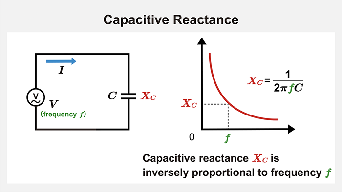
For a capacitor, capacitive reactance (X_C) exhibits the opposite behavior: higher frequencies facilitate easier current flow. It is given by

\(X_C=\displaystyle\frac{1}{2πfC}=\displaystyle\frac{1}{ωC}\)

where C is capacitance.

Reactance forms the imaginary part of impedance. In a purely inductive circuit, current lags the voltage by 90°. In a purely capacitive circuit, current leads the voltage by 90°.

Because inductive and capacitive reactances have opposite signs on the imaginary axis, equal magnitudes cancel each other out.

For more detailed explanations of reactance, concrete circuit examples, and analysis using Bode plots, refer to the dedicated reactance page. See also: Detailed Reactance Page.

Resonant Circuits and Resonant Frequency

In an LC circuit consisting of an inductor and a capacitor, there is a particular frequency at which the magnitudes of inductive and capacitive reactance become equal. This is called the resonant frequency (f₀) and is given by

\(f_0=\displaystyle\frac{1}{2π\sqrt{LC}}\)

In terms of angular frequency, using ω=2πf, we obtain

\(ω_0=\displaystyle\frac{1}{\sqrt{LC}}\)

At resonance, the inductive and capacitive reactances cancel each other out, so the net reactance becomes zero. In a series RLC circuit, the total impedance therefore becomes (approximately) purely resistive, dominated by R at the resonant frequency.

This property is used to implement filters that select a specific frequency and tuning circuits, such as those found in radio tuners.

Impedance Combination Rules and Calculation Methods

When a circuit contains multiple impedances, we must combine them to determine the total impedance. This kind of calculation is frequently required in circuit design and troubleshooting. For example, when several appliances are connected to a household power outlet, we can use impedance calculations to predict the load on the wiring and decide what countermeasures are necessary.

Series Impedance Calculation Methods

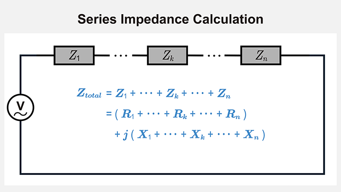
When impedances are connected in series, their total impedance is simply the sum of each element, just like resistors in series:

\(Z_{total}=Z_1+Z_2+Z_3+⋯+Z_n=\displaystyle\sum_{k=1}^{n}Z_k\)

If we separate each element into resistance and reactance, then

\(Z_{total} =(R_1+R_2+⋯+R_n )+j(X_1+X_2+⋯+X_n )\)

\(⟹Z_{total}=\displaystyle\sum_{k=1}^{n}R_k+j\displaystyle\sum_{k=1}^{n}X_k\)

So the sum of all resistive parts becomes the total resistance, and the sum of all reactances becomes the total reactance of the circuit.

As a practical example, consider a series circuit that connects a 10 Ω resistor, a 10 mH inductor, and a 1 μF capacitor at a frequency of 1 kHz.

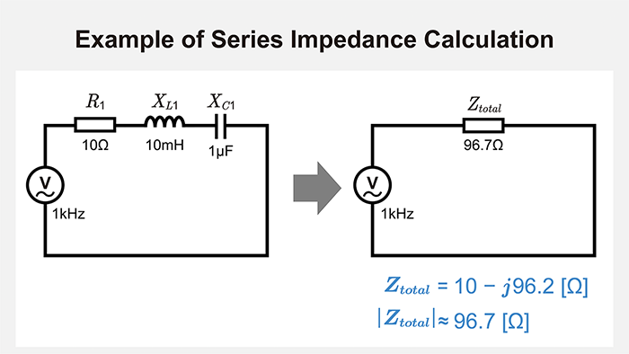
At this frequency, the impedance of each element is

• Resistor: 10+j0 Ω
• Inductor: 0+j62.8 Ω
• Capacitor: 0−j159 Ω

Adding them gives

\(Z_{total} =10+j(62.8-159)=10-j96.2\)

The magnitude of this impedance is

\(|Z_{total}| = \sqrt{10\,^2 + (-96.2)^2} ≈ 96.7\)

Because the imaginary part is negative, the overall circuit exhibits capacitive behavior.

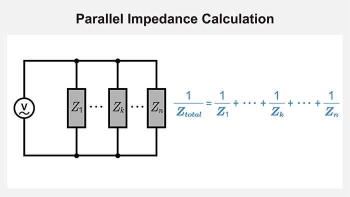
Parallel Impedance Calculation Methods

For impedances connected in parallel, we first add the reciprocals and then take the reciprocal of the sum:

\(\displaystyle\frac{1}{Z_{total}}=\displaystyle\frac{1}{Z_1}+\displaystyle\frac{1}{Z_2}+\displaystyle\frac{1}{Z_3} +⋯+\displaystyle\frac{1}{Z_n}\)

\(⟹Z_{total}=\displaystyle\sum \frac{1}{Z_n}\)

When only two impedances are in parallel, this reduces to the familiar product-over-sum form.

\(Z_{total}=\displaystyle\frac{Z_1 Z_2}{Z_1+Z_2}\)

When the impedances are complex numbers, we must carefully separate real and imaginary parts. As an example, consider two elements

\(Z_1=10+j20\)

\(Z_2=5-j15\)

connected in parallel.

First, we find the admittance (reciprocal) of each impedance:

\(Y_1=\displaystyle\frac{1}{Z_1}=\displaystyle\frac{1}{10+j20}=0.02-j0.04\)

\(Y_2=\displaystyle\frac{1}{Z_2}=\displaystyle\frac{1}{5-j15}=0.02+j0.06\)

Adding them gives the total admittance

\(Y_{total} =Y_1+Y_2=0.04+j0.02\)

Taking the reciprocal yields the total impedance

\(Z_{total}=\displaystyle\frac{1}{Y_{total}}=\displaystyle\frac{1}{0.04+j0.02}\,=20-j10\)

and its magnitude is

\(|Z_{total}|=\sqrt{20\,^2+(-10)^2}\,≈22.36\)

In a purely resistive parallel network, the equivalent resistance is always lower than the smallest individual resistance. However, when imaginary components are present, the result depends on the signs and magnitudes of the reactances, and the magnitude does not necessarily become smaller than each separate element.

Simplifying AC Networks Using Complex Impedance and Thevenin Equivalents

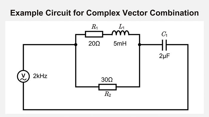
AC circuits often have more complex relationships between elements than DC circuits, making direct analysis tedious. By using series and parallel impedance combinations, we can simplify a complex circuit into an equivalent, more easily analyzed form.

Consider the circuit that operates at 2 kHz shown below: a 20 Ω resistor R₁ and 5 mH inductor are connected in series. This combination is in parallel with a 30 Ω resistor R₂. A 2 µF capacitor C₁ is then connected in series after that parallel network.

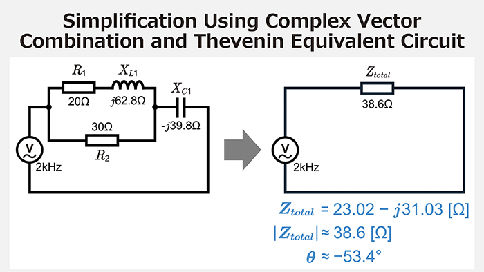
First, we calculate the reactances:

\(X_{L_1}=2π×2000×0.005=62.8\)

\(X_{C_1} = \displaystyle\frac{1}{2π×2000×2×10^{-6}} \,= 39.8\)

The corresponding impedances are

• R₁: 20+j0 Ω
• L₁: 0+j62.8 Ω
• R₂: 30+j0 Ω
• C₁: 0−j39.8 Ω

First we combine R₁ and L₁ in series:

\(Z_{R_1}+Z_L=20+j62.8\)

Next, we combine this result in parallel with R₂. The parallel-combined impedance is

\(Z_2=\displaystyle\frac{(Z_{R_1}+Z_L)Z_{R_2}}{(Z_{R_1}+Z_L)+Z_{R_2}}=\displaystyle\frac{(20+j62.8)×30}{50+j62.8}≈23.02+j8.77\)

Finally, adding the capacitor impedance in series gives the total impedance seen from the load side:

\(Z_{total} =(23.02+j8.77)-j39.8=23.02-j31.03\)

The magnitude and phase angle are

\(|Z_{total}|=\sqrt{23.02\,^2+(-31.03)\,^2}\quad≈38.6\)

\(θ={tan}^{-1}\left(\displaystyle\frac{-31.03}{23.02}\right)≈-53.4°\)

The negative phase angle shows that the overall circuit has capacitive characteristics.

The impedance seen from the load terminals obtained here can be used as the impedance of a Thevenin equivalent circuit. The impedance seen looking into the load terminals can be used as the Thevenin impedance Z_TH. If we also determine the open-circuit voltage at those terminals (the Thevenin voltage V_TH), the original network can be replaced by a simple Thevenin equivalent: a single voltage source V_TH in series with a single impedance Z_TH. In this form, changing the load does not require reanalyzing the entire network, making design iteration more efficient.

For more details on Thevenin’s theorem in DC circuits, please refer to the dedicated page. See also: Detailed Thevenin’s Theorem Page.

Impedance Matching and Transmission Lines

Impedance matching is a technique that improves the efficiency of signal transmission and power transfer by adjusting the impedance of each element in a circuit or system to an optimal value. Proper matching minimizes reflections and losses, thereby optimizing overall system performance.

Input Impedance and Output Impedance

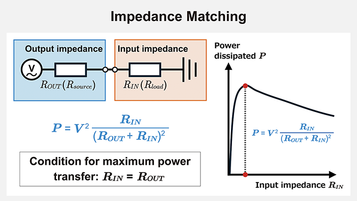
In circuit design, you often encounter the terms “input impedance” and “output impedance.” Input impedance is the impedance seen looking into the input terminals from the signal source. Output impedance is the impedance seen looking back into the source (the device driving the signal).

For example, the compatibility between a music player and a set of headphones depends strongly on the relationship between their output and input impedances.

*For simplicity, the diagram shows only the resistive parts (R_OUT and R_IN). In general, input/output impedance can be complex and frequency-dependent.

Input impedance Z_IN is the impedance at the input terminals as seen from the signal source:

\(Z_{IN} =\displaystyle\frac{V_{IN}}{I_{IN}}\)

A high input impedance loads the source less and helps prevent distortion and loss of the input signal. For AC signals, the value may change depending on frequency.

Output impedance Z_OUT is the internal impedance of the device that sends out the signal. In general, it is a complex quantity that can be written as Z_OUT = R_OUT + jX_OUT. If X_OUT > 0, the output appears inductive, and if X_OUT < 0, it appears capacitive. To determine Z_OUT, we can use the open-circuit voltage V_open (no load connected), along with the load voltage V_load and load current I_load when a load is attached:

\(Z_{OUT} = \displaystyle\frac{V_{open}-V_{load}}{I_{load}}\)

When considering power transfer, the maximum power transfer theorem states that (in sinusoidal steady state) maximum average power is delivered when the load impedance equals the complex conjugate of the source (Thevenin) impedance:

\(Z_L=Z_{OUT}^*\)

Here,(·)^*denotes complex conjugation; if Z = a + jb, then Z* = a − jb. If we further assume a purely resistive case (or that reactive components are cancelled by a matching network), the average load power reduces to:

\(P=\displaystyle\frac{V_{TH}^2 R_{IN}}{(R_{OUT}+R_{IN})^2}\)

where V_TH is the RMS Thevenin voltage at the load terminals (open circuit), R_OUT is the resistive part of the source (output) impedance, and R_IN is the load resistance. From this expression, power is maximized when R_IN = R_OUT.

However, under the maximum-power-transfer condition, the same amount of power is dissipated in the source’s internal resistance, so the efficiency is limited to 50%. Therefore, this condition is most often used when the goal is not efficiency but reflection control and a well-defined system impedance, such as in RF and transmission-line systems (e.g., 50 Ω/75 Ω environments). In many low-frequency audio and instrumentation interfaces, the design goal is usually voltage transfer rather than maximum power transfer, so the source impedance is designed to be much lower than the load impedance.

In many practical designs, impedance matching is an important design consideration.

For instance, microphones typically have a low output impedance (approximately 50–600 Ω) and are connected to audio amplifiers with a high input impedance (10 kΩ or higher) so that the source is not heavily loaded and the signal voltage is preserved.Likewise, when a power amplifier drives a loudspeaker (4–16 Ω), the amplifier is typically designed with a very low output impedance (well below 1 Ω) so that the speaker is driven close to a constant-voltage source. This improves damping (control of the driver) and reduces frequency-response variation caused by the speaker’s impedance curve.

Impedance Measurement Methods and Troubleshooting

Even a circuit that is perfectly correct on paper may not produce the expected values when actually powered and measured. Impedance is a powerful clue for identifying the leading causes of such discrepancies, but the measured value is sensitive to the measurement method and environmental conditions. Here, we summarize why measurement is necessary, the instruments used, and the types of problems that often occur.

Need for Impedance Measurement

The impedance calculated at the design stage can change significantly due to component tolerances, parasitic elements in the wiring, and environmental factors such as temperature and humidity. Only by actual measurement can we see the true circuit characteristics and separate the contributions of various error sources. Using measured data as a reference, you can re-select components, adjust wiring layout, and obtain concrete assurance that the finished product will operate stably.

Types of Measurement Methods

For quickly checking the values of individual components at low frequencies, an LCR meter is a convenient tool. For slightly higher frequencies and more detailed tracking of changes, an impedance analyzer is an effective tool. For evaluating transmission lines and antennas in the gigahertz range, a vector network analyzer (VNA) is indispensable. Selecting the appropriate instrument according to the target frequency band and required accuracy has a significant impact on measurement quality.

Common Troubles During Impedance Measurement

If measured values fluctuate, poor contact of probes or fixtures is often the cause. Rusty terminals or loose clips alter the contact resistance, making the results unstable. When measuring high-gain amplifiers or high-frequency modules, the measurement system itself can become unstable and oscillate. Environmental electromagnetic noise and temperature variations can also have a significant impact. Many of these problems can be mitigated by shielding instruments, keeping cables short and tidy, and maintaining stable environmental conditions.

Impedance Summary

In this article, we examined impedance, a key quantity in AC circuit analysis. Impedance represents the overall opposition to AC current flow in a circuit, combining resistance with the reactance of inductors and capacitors. Because impedance is strongly affected by frequency, AC circuits require different treatment from DC circuits.

By understanding the difference between resistance and reactance, how they combine in series and parallel, and how resonant behavior arises, you gain practical knowledge for circuit design and troubleshooting in many kinds of electrical and electronic equipment. We also discussed the roles of input and output impedance, as well as the basic concepts of impedance matching, which are crucial for efficient power transfer and high-quality signal transmission. Finally, we discussed the importance of using proper measurement methods and maintaining environmental control to obtain accurate impedance data.

A solid grasp of impedance fundamentals enhances predictability during the design stage and facilitates precise responses when problems arise in actual hardware.

Related article

Electrical Reactance

What Is Thevenin’s Theorem?: DC Circuit Analysis