Kirchhoff's laws describe how current and voltage are related throughout an electric circuit. There are two of them: Kirchhoff's current law (KCL), which governs the currents entering and leaving a node, and Kirchhoff's voltage law (KVL), which governs the voltages around a closed loop.
If you have ever analyzed a simple circuit, you have used Ohm's law. It works beautifully for a single source and a single path. But the moment a circuit branches, or a second source appears, Ohm's law alone can no longer determine every unknown current and voltage. The standard approach in that situation is to write equations using Kirchhoff's laws and solve them as a system of simultaneous equations. Every circuit simulator and every engineer doing hand analysis relies on this procedure.
This article covers the formulas, when to use each law, and how to assign signs correctly, which is where most mistakes happen. It then works through three examples in full: the current at a node, the voltage drops in a series circuit, and a circuit with two sources. Each example is solved through the numbers and verified with a check calculation, so you can confirm your own work the same way.
Kirchhoff's Law Formulas at a Glance
If you came here for the formulas, here they are. The rest of the article explains how to apply them without sign errors.
| Law | Formula | Meaning |
|---|---|---|
| Kirchhoff's current law (KCL) | \(\sum I_{IN}=\sum I_{OUT}\) | The sum of currents entering a node equals the sum of currents leaving it |
| Kirchhoff's voltage law (KVL) | \(\sum V=0\) | The sum of voltages around any closed loop is zero |
KCL organizes the currents at a point (a node). KVL organizes the voltages around a path (a closed loop). Keeping that point-versus-path distinction in mind is the fastest way to decide which law applies to a problem, and the next table makes the decision explicit.
KVL vs. KCL: When to Use Which
| Situation | Law to use | How the equation works |
|---|---|---|
| Current splits or merges at a node | Kirchhoff's current law (KCL) | Sum of currents in = sum of currents out |
| Tracking voltages around one loop | Kirchhoff's voltage law (KVL) | Voltages around the loop sum to zero |
| Several nodes to solve at once | Nodal analysis | Apply KCL at each node |
| Several loops to solve at once | Mesh analysis | Apply KVL around each loop |
When in doubt: if you are looking at a point, use KCL; if you are going around a loop, use KVL. Real problems usually need both, one KCL equation per independent node and one KVL equation per independent loop, which is exactly what Example 3 will demonstrate. First, though, it is worth seeing why each law is true, because the reasoning is what makes the sign rules feel natural rather than arbitrary.
What Are Kirchhoff's Laws?
Kirchhoff's laws are the collective name for two laws formulated by the German physicist Gustav Kirchhoff in 1845: the first law, which concerns current, and the second law, which concerns voltage. These laws are not special rules created only for circuits. The first law applies the conservation of charge to a junction in a circuit, while the second law applies the conservation of energy to a closed path. Because Kirchhoff's laws are based on fundamental principles of physics, they are widely used as a starting point for circuit analysis. In this chapter, we will review the first and second laws in order, using diagrams and equations.
Kirchhoff's Current Law (KCL)
KCL states that the total current flowing into a node equals the total current flowing out of it:
\(\sum_{}^{}I_{in}=\sum_{}^{}I_{out}\)
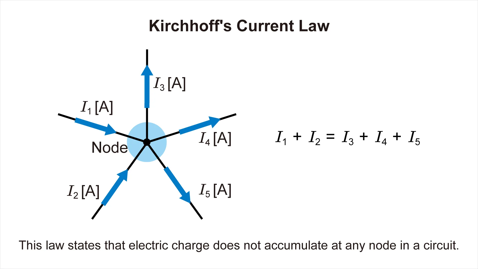 Figure 1. Currents entering and leaving a node (KCL)
The law holds because charge cannot pile up at a node. A wiring junction is just a connection point. It has no capacity to store charge, so whatever current arrives must leave at the same rate. Picture a tee fitting in a water pipe: the water flowing in through two branches has nowhere to go but out through the third.
You can state the same law in a second way that is often more convenient for writing equations: take inflow as positive and outflow as negative, and the algebraic sum of currents at a node is zero. Both forms appear in textbooks, and they are interchangeable.
Kirchhoff's Voltage Law (KVL)
KVL states that the sum of all voltages around a closed loop is zero:
\(\sum_{}^{}V=0\)
![Diagram of Kirchhoff's voltage law (KVL) showing that the source EMF and the voltage drops across resistors around a closed loop sum to zero]](https://techweb.rohm.com/wp-content/uploads/2026/09/img21777-02-image_2.webp) Figure 2. Voltages around a closed loop (KVL)
Figure 2. Voltages around a closed loop (KVL)
The reasoning here is the conservation of energy. Voltage is electric potential, and potential is a property of position in the circuit. If you travel around a loop and return to your starting point, the potential must return to its starting value, so every rise in potential along the way (through a source) is exactly canceled by the falls (across resistors and other loads). Equivalently: the sum of the EMFs around a loop equals the sum of the voltage drops.
This balance is worth internalizing because it is also a physical statement. The energy a source feeds into the loop is exactly the energy the loads consume. We will use that fact at the end of Example 3 to double-check a solution through its power balance.
Choosing Between KCL and KVL
The two laws apply to different objects. KCL describes the currents at a point, the node. KVL describes the voltages around a path, the closed loop. If the unknown is a branch current after a split, start with KCL. If it is the voltage across each component, start with KVL. When a circuit has several unknowns, write a KCL equation for each independent node and a KVL equation for each independent loop, then solve the set simultaneously. That sounds abstract on first reading, so the three examples below build up the procedure one step at a time, from a single node to a full two-source network.
How to Set Up the Equations: Sign Conventions
The hardest part of Kirchhoff's laws is not the laws themselves. It is keeping the signs straight, and nearly every wrong answer in circuit analysis traces back to a sign slip. The good news is that signs stop being a problem once you follow a fixed routine. Use these five steps in the same order every time.
- Assume a direction for the current in each branch and draw the arrows on the circuit diagram.
- Choose a direction to travel around each loop (clockwise, for example) and keep it fixed for that loop.
- Travel around the loop, adding each voltage as positive where the potential rises and negative where it falls.
- For a resistor, if you pass through it in the same direction as the assumed current, count it as a voltage drop (negative).
- Set the total for the full loop equal to zero.
Two of these steps deserve a comment. In step 1, the assumed directions do not need to be correct. If an assumption turns out to be wrong, the answer for that current becomes negative, and the calculation still works; we will see exactly this in the section on negative answers. In step 3, notice that you never need separate rules for sources and resistors. One question handles everything: ask whether the potential rises or falls in your direction of travel.
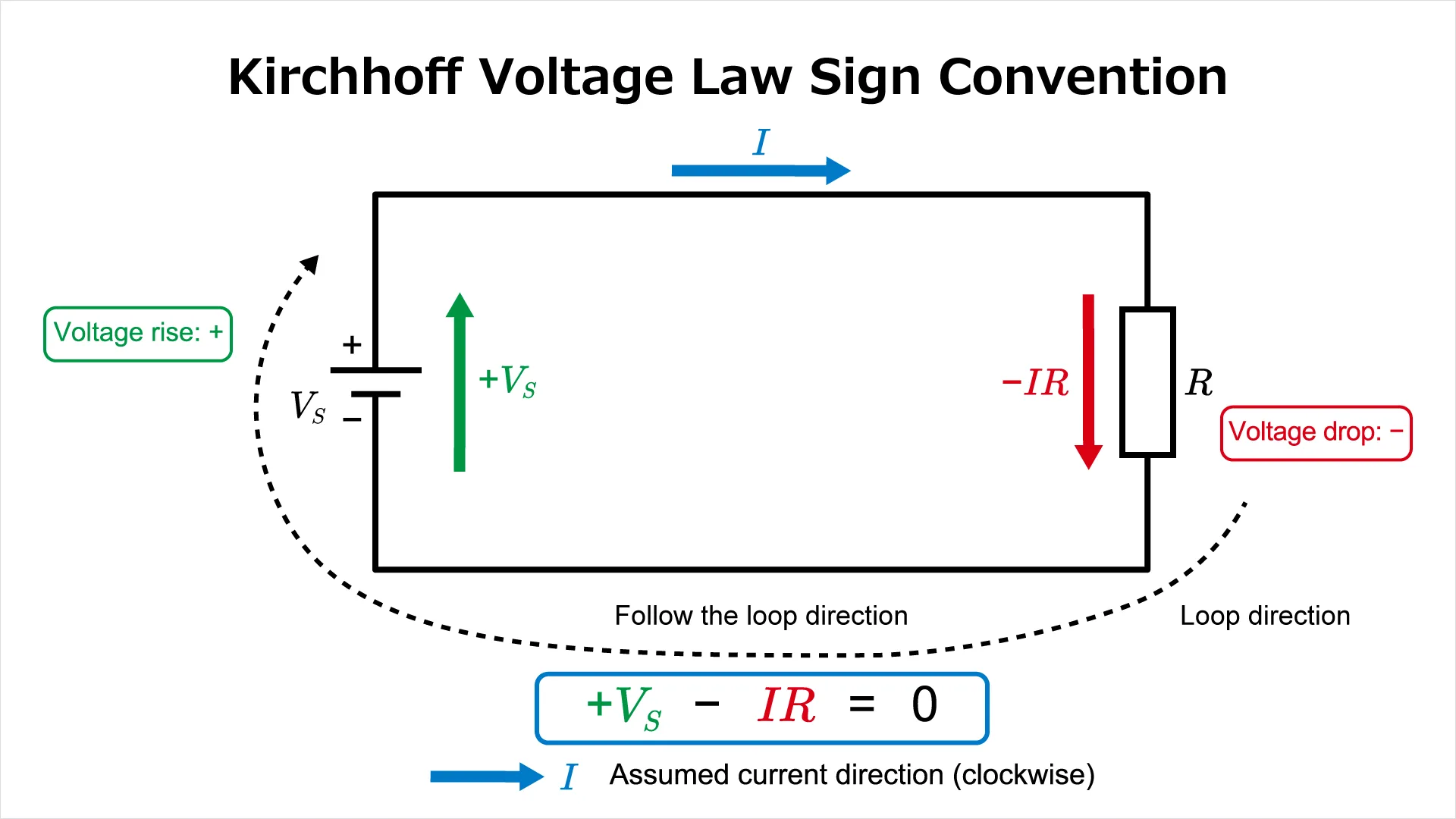 Figure 3. A loop annotated with current arrows and signs
Here is the routine applied to the simplest possible case: a source \(V_{S}\) driving three resistors in series. Assume the current flows out of the positive terminal and travels around the loop in that same direction. Passing through the source from its negative terminal to its positive terminal, the potential rises, so the source contributes + \(V_{S}\). Passing through each resistor in the direction of the current, the potential falls, so each contributes a negative term:
\(V_{S}-V_{1}-V_{2}-V_{3}=0\)
Moving the voltage drops to the right-hand side:
\(V_{S}=V_{1}+V_{2}+V_{3}\)
Read in words, the second form says the source voltage equals the sum of the voltage drops, which is the "EMFs equal voltage drops" statement from earlier. The two forms are the same equation rearranged. Textbooks use both, and you can write whichever feels clearer for the problem at hand.
Example 1: Finding the Current at a Node
We will start with the smallest possible problem, one node and one application of KCL. This is the situation at every junction on a circuit board: several traces meet, and you know some of the currents but not all of them.
Problem:
Currents \(I_{1}\)=2A and \(I_{2}\)=3A flow into a node, and current \(I_{3}\) flows out. Find \(I_{3}\).
![Example for Kirchhoff's current law: currents of 2A and 3A enter a node and a single current I_3 leaves it]](https://techweb.rohm.com/wp-content/uploads/2026/09/img21777-04-image_4.webp) Figure 4. Node with two currents in and one current out
Figure 4. Node with two currents in and one current out
Solution:
Two quantities are known: the two inflowing currents. One is unknown, the outflow. KCL connects them directly because the current flowing in must equal the current flowing out:
\(I_{1}+I_{2}=I_{3}\)
\(2+3=I_{3}\)
\(I_{3}=5A\)
If you prefer the algebraic-sum form, write inflow as positive and outflow as negative: 2+3-\(I_{3}\)=0, which gives the same answer.
The basic use of the first law can be understood from what has been shown so far. Even as a circuit becomes larger and the number of nodes increases, the basic approach remains the same: organize the currents entering and leaving each node. By writing equations of the same form for the necessary nodes and solving them simultaneously, the currents in each part of the circuit can be determined. When this is combined with the second law, it becomes possible to analyze an entire circuit, including resistors and power sources, more systematically.
Example 2: Finding the Voltage Drops in a Series Circuit
Next, one loop and one application of KVL. This is also a first look at how Kirchhoff's laws and Ohm's law divide the labor: KVL sets up the loop equation, and Ohm's law expresses each resistor's voltage in terms of the current.
Problem:
A 12 V source is connected to a 3 Ω resistor and a 5 Ω resistor in series. Find the current and the voltage drop across each resistor.
![Example circuit for Kirchhoff's voltage law: a 12 V source in series with 3-ohm and 5-ohm resistors carrying a current of 1.5 A]](https://techweb.rohm.com/wp-content/uploads/2026/09/img21777-05-image_5.webp) Figure 5. A series circuit with a 12 V source, 3 Ω, and 5 Ω |
Figure 5. A series circuit with a 12 V source, 3 Ω, and 5 Ω |
Solution:
In a series loop there is only one current, so call it I and assume it flows out of the positive terminal of the source. Travel around the loop in that direction. The source is a rise of 12V; each resistor, by Ohm's law, is a drop of (\(I \times R\)):
\(12-3I-5I=0\)
Collect the current terms and solve:
\(8I=12\)
\(I=1.5A\)
With the current known, Ohm's law gives each voltage drop:
Across 3Ω:
\(V_{1}=1.5 \times 3=4.5V\)
Across 5 Ω:
\(V_{2}=1.5 \times 5=7.5V\)
Check:
\(V_{1}+V_{2}=4.5+7.5=12V\)
which matches the source voltage exactly. If the drops do not add up to the source voltage, a sign or an arithmetic step is wrong somewhere, and it is far cheaper to catch that now than after the result has been used.
Notice what the numbers are telling you. The 12 V is divided between the resistors in proportion to their resistances: 4.5 V and 7.5 V across the 3 Ω and 5 Ω resistors, respectively. That proportional split is the voltage divider, one of the most used relationships in practical electronics, and it is nothing more than this example generalized.
Example 3: Solving a Circuit with Two Sources
This is where Kirchhoff's laws earn their keep. With two sources driving the same network, you cannot reduce the circuit by combining series and parallel resistances, because no single source "owns" the current distribution. Kirchhoff's laws handle it without any special technique: count the unknowns, write that many independent equations, and solve.
Problem:
Three branches connect an upper node A to a lower common rail:
- Branch 1: source \(V_{S1}\)=12V in series with resistor \(R_{1}\)=2Ω
- Branch 2: resistor \(R_{2}\)=4Ω
- Branch 3: resistor \(R_{3}\)=2Ω in series with source \(V_{S2}\)=6V
For both \(V_{S1}\) and \(V_{S2}\), the positive terminal faces node A (the upper side) and the negative terminal faces the lower common rail. The source polarities follow the orientation shown in the figure. Find the current in each branch.
![Example circuit with two sources solved using Kirchhoff's laws, showing a 12 V source, a 6 V source, three resistors, node A, branch currents I_1, I_2, and I_3, and the polarity of each source]](https://techweb.rohm.com/wp-content/uploads/2026/09/img21777-06-image_6.webp) Figure 6. A circuit with two sources and three resistors
Figure 6. A circuit with two sources and three resistors
Step 1: Count the unknowns and assume directions.
There are three branches, so there are three unknown currents. We therefore need three independent equations. Assume the directions first: let \(I_{1}\) flow from branch 1 into node A, \(I_{2}\) flow from node A down through \(R_{2}\), and \(I_{3}\) flow from node A through \(R_{3}\) into branch 3. These are guesses, and that is fine. Any current we guessed backwards will simply appear with a minus sign.
Step 2: Apply KCL at node A.
Current in equals current out:
\(I_{1}=I_{2}+I_{3}\)
That is one equation. Two to go.
Step 3: Apply KVL to two loops.
After obtaining the currents, check that the results are consistent with the circuit as a whole. The first check uses the outer loop, which was not used when setting up the equations.
Going around the outer loop in the direction \(V_{S1}\) → \(R_{1}\) → \(R_{3}\) → \(V_{S2}\), the voltage rise caused by \(V_{S1}\) balances the voltage drops across \(R_{1}\), \(R_{3}\) and \(V_{S2}\). Therefore, from KVL, the following equation holds:
\(V_{S1}-R_{1}I_{1}-R_{3}I_{3}-V_{S2}=0\)
Substitute \(V_{S1}\)=12 V, \(R_{1}\)=2 Ω, \(I_{1}\)=2.4 A, \(R_{3}\)=2 Ω, \(I_{3}\)=0.6 A, and \(V_{S2}\)=6 V:
\(12-2 \times 2.4-2 \times 0.6-6=12-4.8-1.2-6=0\)
Since KVL also holds for the outer loop, the calculated currents are consistent with the voltage relationships in the circuit.
The second check is the power balance. Because KVL is based on the conservation of energy, the power supplied and the power consumed or absorbed must also balance in the circuit as a whole.
The power supplied by the 12 V source is the product of the source voltage and the current flowing out of the source.
\(P_{S1}=V_{S1}I_{1}\)
\(P_{S1}=12 \times 2.4=28.8 W\)
On the other hand, the power dissipated by the three resistors can be calculated from \(P=I^{2}R\):
\(P_{R}=I_{1}^{2}R_{1}+I_{2}^{2}R_{2}+I_{3}^{2}R_{3}\)
\(P_{R}=2.4^{ 2} \times 2+1.8^{ 2} \times 4+0.6^{ 2} \times 2=11.52+12.96+0.72=25.2 W\)
The 12 V source supplies 28.8 W, while the resistors dissipate 25.2 W. The difference, 3.6 W, is absorbed by the 6 V source.
In this circuit, \(I_{3}\) flows into the positive terminal of \(V_{S2}\). Therefore, the 6 V source absorbs power instead of supplying it.
\(P_{S2}=V_{S2}I_{3}\)
\(P_{S2}=6 \times 0.6=3.6 W\)
Therefore, the sum of the power dissipated by the resistors and the power absorbed by the 6 V source is:
\(25.2+3.6=28.8 W\)
This matches the power supplied by the 12 V source. Thus, the calculated currents are valid not only from the voltage relationships but also from the power balance of the circuit.
Common Mistakes and What a Negative Answer Means
The procedure above is reliable, but a few habits trip up almost everyone at first. Most errors with Kirchhoff's laws fall into four patterns, and all four are avoidable.
- Changing an assumed current direction partway through. Once you draw arrows, leave them alone until the answer is out. If a direction changes from one equation to the next, the signs fall apart and no amount of careful algebra can save the result.
- Mixing up the signs of voltage drops and EMFs. Judge every element by the same question: ask whether the potential rises or falls in your direction of travel. Then there is nothing separate to memorize for sources versus resistors.
- Treating a negative answer as a calculation error. A negative result means only that the actual current flows opposite to the assumed direction. The magnitude is correct as is. Suppose that in Example 3 we had assumed \(I_{3}\) pointing the other way, from branch 3 into node A. Every step would proceed the same, and the answer would come out \(I_{3}\)=−0.6A: same current, same physical direction, reported against a reversed reference. Flip the arrow in your head and move on.
- Assuming parallel branches carry the same current. What parallel branches share is the voltage. The currents differ from branch to branch, and KCL is what determines how they divide.
The single best defense is the one used in both examples: substitute the solved values into a loop you did not use when setting up the equations and confirm that the KVL sum is zero. The check takes seconds and catches most sign errors on the spot.
Loops, Closed Circuits, and Open Circuits
Every example above involved going "around a closed loop," and so far we have relied on intuition to understand what that means. The intuition is usually enough, but three related terms are worth pinning down precisely, because one common situation, the open circuit, is where loose terminology leads to wrong conclusions.
![Comparison of an open circuit, where an open switch stops the current, and a closed circuit, where the completed path carries current]](https://techweb.rohm.com/wp-content/uploads/2026/09/img21777-07-image_7.webp) Figure 7. Open circuit and closed circuit
Figure 7. Open circuit and closed circuit
Loops vs. Closed Circuits
A loop (a closed loop) is any path on the circuit diagram that you can trace continuously back to its starting point. KVL applies to any loop, whether or not current actually flows through it. A closed circuit, by contrast, is a loop that actually carries current: a complete path from the source through resistors, capacitors, inductors, or other elements and back to the source. In a closed circuit, current flows continuously and the voltage drops are distributed across the elements along the path.
In everyday circuit analysis you can usually ignore the distinction. It starts to matter once an open circuit is involved.
Open Circuits and KVL
An open circuit is a state in which the current path is interrupted by an open switch or a broken wire, so no current flows.
Here is the point that surprises many learners: even if a loop contains a branch carrying no current, KVL still holds as long as you can trace the loop. In a loop containing an open switch, the current is zero, so the voltage drops across the resistors are zero too. A potential difference, however, remains across the switch terminals, and the algebraic sum of voltages around the loop, including that potential difference, still comes to zero. In fact, with every resistor dropping zero volts, the full source voltage appears across the open switch.
This is not a technicality. It lets you calculate the voltage across an open switch or the potential difference at a break in a wire, which is the daily bread of failure analysis. When a board stops working, the full supply voltage showing up across an unexpected gap is often exactly how you find the broken trace. The same reasoning applies when designing switching circuits that create open circuits on purpose.
Relate to Ohm's Law, Mesh and Nodal Analysis
Kirchhoff's laws are not standalone tools. To relate the voltage and current of each resistor, they must be used together with Ohm's law. As circuits become larger, they evolve into systematic solution methods known as mesh analysis and nodal analysis.
However, Kirchhoff's laws cannot be applied unconditionally to every circuit. There is one fundamental assumption that must be satisfied for them to hold. In this chapter, we position Kirchhoff's laws within the practical map of circuit analysis.
Once you see the overall picture, it becomes clear that the analysis methods you will study later are all extensions of Kirchhoff's laws. This makes it much easier to understand where your learning is heading.
Combining with Ohm's Law
Ohm's law relates the voltage V, current I, and resistance R of a conductor:
\(V=I \times R\)
Kirchhoff's laws describe how currents and voltages connect throughout the circuit, while Ohm's law relates voltage and current at each resistor. The division of labor was evident in both worked examples: KVL provided the loop equation, and Ohm's law turned each resistor's voltage into \(I \times R\), reducing the unknowns to currents alone. The two laws never compete; they are always used together. For a full treatment of Ohm's law itself, see the Ohm’s law article.
DC and AC Circuits
In DC circuits, the current direction and voltages are constant, so KCL and KVL apply exactly as described above. In AC circuits, voltage and current vary with time, and phase and frequency come into play, so the same laws are applied using impedance in place of resistance. The laws themselves still hold for AC; the arithmetic involves complex numbers, but nothing about the loop-and-node reasoning changes.
One boundary is worth knowing. Kirchhoff's laws hold when the circuit can be treated as a lumped-element circuit: a model in which each property, such as resistance or source voltage, is concentrated in its component and the wiring itself can be neglected. As signal frequencies rise and trace lengths become significant compared with the wavelength, that model breaks down and the circuit must be treated with distributed-element methods. For power circuits and low-frequency signals, this almost never comes up, but for high-speed or high-frequency board design, knowing where the lumped-element assumption ends is the starting point for layout decisions.
From Kirchhoff's Laws to Mesh and Nodal Analysis
As the number of loops and nodes grows, writing equations one at a time becomes tedious and error-prone. Mesh analysis applies KVL systematically to every loop, and nodal analysis applies KCL systematically to every node, each with a fixed bookkeeping scheme that keeps the signs organized for you. Both are Kirchhoff's laws expressed as procedures, so if you followed Example 3, you already understand their foundations. For circuits with four or more unknowns, continue to the mesh analysis and nodal analysis articles.
Measuring Voltage and Current with Kirchhoff's Laws
Kirchhoff's laws are not only for paper analysis. They are also the basis for judgment when measuring real circuits, both for deciding where to probe and for interpreting what the instruments report.
To measure voltage, connect a voltmeter in parallel across the two points of interest. Once a few voltages in a loop have been measured, the remaining unknown voltages can be calculated from KVL. This is why, on a board where not every point can be probed, the voltages you cannot reach can still be estimated from the ones you can.
![Voltage measurement diagram showing a voltmeter connected in parallel across the two points being measured]](https://techweb.rohm.com/wp-content/uploads/2026/09/img21777-08-image_8.webp) Figure 8. Voltmeter connected in parallel
Figure 8. Voltmeter connected in parallel
To measure current, connect an ammeter in series with the branch of interest. In a circuit with branches, measuring the current at one point is often enough because KCL determines the currents in the other branches and reduces the number of measurement points.
![Connection diagram for current measurement. The ammeter is connected in the section where the current is to be measured.]](https://techweb.rohm.com/wp-content/uploads/2026/09/img21777-09-image_9.webp) Figure 9. Ammeter Connected in Series
Figure 9. Ammeter Connected in Series
The laws also serve as a sanity check on the measurements themselves. If readings contradict KCL or KVL, something is wrong with either the measurement setup or the circuit, and that contradiction is useful information. For detailed measurement techniques, see the article on current and voltage in DC circuits.
Potential Difference and EMF: The Physics Behind KVL
To close the technical discussion, here are the two concepts behind the voltage law, which explain why KVL is an energy statement and not merely a bookkeeping rule.
Potential difference is the difference in electric potential (the level of electrical energy) between two points. If moving a charge Q from one point to the other takes work W, the potential difference V is:
\(V=W/Q\)
The unit is the volt (V).
Electromotive force (EMF) is the potential difference that a source, such as a battery or generator, creates in a circuit. It arises as the field inside the source pushes charge to a higher potential, and it represents the source's capacity to supply energy to the circuit.
With these two concepts, KVL's \(\sum V=0\) reads as: the sum of the EMFs equals the sum of the voltage drops. The energy supplied by the sources and the energy consumed by the loads balance exactly over one trip around any closed circuit. That is the balance we verified numerically in Example 3's power check, and it is the place to start whether you are budgeting supply voltages in a design or chasing down where the voltage is being lost in a failing board.
Key Takeaways
- Kirchhoff's current law (KCL): the currents into a node equal the currents out, \(\sum I_{IN}=\sum I_{OUT}\).
It is the conservation of charge at a junction. - Kirchhoff's voltage law (KVL): the voltages around any closed loop sum to zero, \(\sum V=0\).
It is the conservation of energy around a path, and it holds even for loops that carry no current. - Use KCL at points and KVL around loops. For circuits that series-parallel reduction cannot handle, such as circuits with two sources, write one equation per independent node and loop and solve them together..
- Assume current directions freely and never change them mid-problem.
A negative answer is not an error; it means the real current flows opposite to your arrow. - Always verify: substitute the solution into an unused loop and confirm the KVL sum is zero.
For full confidence, check the power balance as well.
Once these habits are in place, the natural next step is to let the bookkeeping scale for you. The mesh analysis and nodal analysis articles take the same two laws and turn them into systematic procedures for larger circuits.