Norton’s Theorem: Equivalent Circuit Analysis

Norton’s theorem is very useful for simplifying electric circuit analysis. Even in complex circuits, if you focus on two specific terminals, you can express the circuit with a current source in parallel with a single resistor. For example, Norton’s theorem helps you efficiently find the current or voltage at a connected load in circuits containing voltage sources, resistors, or even dependent sources. From basic electrical studies to more specialized fields of electronics, it is widely applied and frequently introduced in textbooks and design references. Here, we will explain the fundamental ideas behind Norton’s theorem, how its proof works, concrete steps to find the equivalent circuit, and a comparison with Thevenin’s theorem.

Fundamental Principle of Norton’s Theorem

Norton’s theorem states that “any complex linear circuit, when viewed from a pair of terminals, can be replaced by a single current source (I_N) in parallel with a single resistor (R_N).”

A “linear circuit” is one where the voltage and current remain linear. It typically involves resistors, linear independent sources, and dependent sources. Suppose nonlinear components such as diodes or transistors are present. A linearized equivalent circuit can sometimes be applied near a specific operating point, although this article focuses primarily on linear elements.

One advantage of Norton’s theorem is that you can focus only on the terminal where the load is attached, transforming the complicated circuit into just two elements. Ultimately, this simplifies calculations of the load current and the voltage across the load resistance at those terminals, making it convenient for designers and students.

Components of the Norton Equivalent Circuit

To apply Norton’s theorem effectively, you must understand precisely what elements make up the equivalent circuit. A Norton equivalent circuit consists of just two parts: a current source and a parallel resistance (R_N). Recognizing this structure helps you quickly grasp the essential details of even a complex-looking circuit. Below, we explain the elements central to Norton’s theorem, such as the Norton current and the Norton resistance, and how they interact.

Norton Current

When you apply Norton’s theorem, you end up with an ideal current source labeled I_N. By definition, I_N is the current flowing when you short-circuit (directly connect) the two terminals under consideration.

Specifically, you replace the load resistor with an ideal conductor and calculate or measure how much current flows into that shorted connection.

An ideal current source supplies a constant current I_N regardless of the terminal voltage. Although fundamental circuit elements do not have infinite internal resistance, this idealization helps simplify calculations and clarify the interaction with the load.

Norton Resistance

Alongside the current source, Norton’s theorem includes a single resistor R_N in parallel.

R_N is determined by setting all independent circuits’ sources to zero (replace voltage sources with short-circuits and current sources with open circuits) and then measuring or calculating the two-terminal resistance you observe. If there are dependent sources, you must leave them in place because their outputs depend on other parts of the circuit. If only dependent sources remain after zeroing all independent sources, insert a test source across the two terminals (for example, a 1 V voltage source or a 1 A current source) and compute.

\(R_N=\displaystyle \frac{V_{test}}{I_{test}}\)

with the dependent sources active. This guarantees the correct two-terminal resistance even when passive combination alone is not possible.

R_N is crucial because it determines how the current source interacts with the load. From the viewpoint of parallel connection, the load resistor is placed in parallel with R_N, directly affecting load voltage calculations or load current.

A Schematic of the Norton Equivalent Circuit

The Norton equivalent circuit can be represented by a simple Norton’s theorem circuit diagram: a single current source (I_N) in parallel with a single resistor (R_N). The output terminals of these two elements correspond to the original circuit’s load connection.

Visually, imagine a current source at the top and a resistor at the bottom, both in parallel, with the load resistor attached to the right. Although this shape is different from the Thevenin equivalent circuit (which uses a voltage source V_Th in series with R_Th), the two forms can be converted into each other.

Finding Norton Current and Norton Resistance

When applying Norton’s theorem, the most important steps involve calculating the Norton current (I_N) and the Norton resistance (R_N). Once you know how to determine the short-circuit current and zero out all independent sources to find the resistance, you can analyze many linear circuits. Here we discuss these steps in order and illustrate the calculations with examples.

How to Calculate the Norton Current

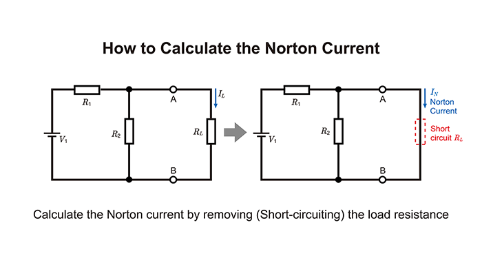
1. Short the two terminals you are analyzing.
   In simpler terms, replace the load resistor R_L with a direct wire connection.
2. Use circuit equations or analysis to determine the current flowing through that short-circuit.
   You may use Kirchhoff’s laws (KCL, KVL), Ohm’s law, or superposition.
3. That short-circuit current is I_N.
   This value becomes the ideal current source in your Norton equivalent circuit.

Example Equations

Consider a straightforward circuit with a single voltage source V_S in series with a resistor R_S, feeding a load resistor R_L. If you short the terminals where R_L was, the circuit is simply V_S in series with R_S, making the short-circuit current:

\(I_{SC} = \displaystyle \frac{V_S}{R_S}\)

Hence,

\(I_N=I_{SC}=\displaystyle \frac{V_S}{R_S}\)

If there are multiple sources, you can apply superposition to each source’s contribution, then sum to find I_N.

How to Calculate the Norton Equivalent Resistance

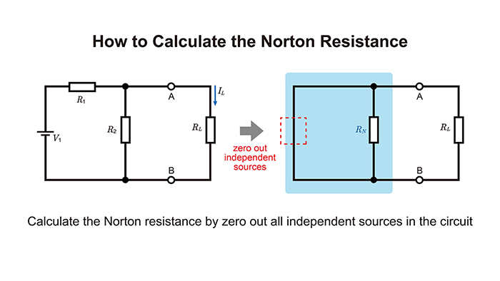
1. Zero out all independent sources in the circuit.
   Replace voltage sources with short-circuits and current sources with open circuits.
   If there are dependent sources, keep them since they depend on other signals in the circuit.
2. Determine the resistance seen from the same two terminals.
   You might combine series and parallel resistors or do node analysis.
3. This resistance is R_N.
   It represents the parallel resistor in the Norton equivalent circuit.

Example Equations

In the simple case above, if you short the voltage source V_S (i.e., set it to zero), then R_S is directly seen at the two terminals. Therefore:

\(R_N=R_S\)

For more complex resistor networks, you systematically combine or analyze them to find the final resistance.

Circuit Analysis Example

Understanding Norton’s theorem conceptually is one thing, but seeing how it works in calculations or simulations is another. In this section, we show a circuit with multiple sources and resistors, and go step by step to find the Norton equivalent. This process will clarify how to apply the theorem in real practice, including analyzing load resistor voltage under various source and load conditions.

Example Setup

• There is a voltage source V₁ with internal resistor R₁, and another V₂ with internal resistor R₂.
• These combine at some node, which connects to the load resistor R_L.
• Additionally, another resistor R₃ connects that same node to ground.
• We removed R_L and considered those two terminals for the Norton equivalent.

Though this may seem complicated in text, it’s a typical example of multiple sources and resistors.

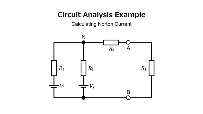
Calculating Norton Current

1. Draw the circuit with the load R_L replaced by a short-circuit.
2. Identify how V₁, R₁, V₂, R₂, and R₃ connect at the short-circuit point.
3. Apply KCL and KVL, or superposition, to solve for the unknown currents.
4. The sum of the currents flowing into that shorted node is your Norton current I_N.

Example equations might look like this:

Label the short-circuit node voltage as V_SC. Then

\(I_1=\displaystyle \frac{V_1-V_{SC}}{R_1}, I_2=\displaystyle \frac{V_2-V_{SC}}{R_2}, I_3=\displaystyle \frac{V_{SC}}{R_3}\)

KCL at the short-circuit node gives I₁+I₂=I₃. Solving yields

\(V_{SC}=\displaystyle \frac{ \displaystyle \frac{V_1}{R_1} + \displaystyle \frac{V_2}{R_2}}{\displaystyle \frac{1}{R_1} + \displaystyle \frac{1}{R_2} + \displaystyle \frac{1}{R_3}}\)

and therefore the Norton current

\(I_N=I_3=\displaystyle \frac{V_1 R_2+V_2 R_1}{R_1 R_2+R_2 R_3+R_1 R_3}\)

Then KCL at the short-circuit node is:

\(I_1+I_2=I_3\)

Solving for V_SC gives you the individual currents, and IN is the total short-circuit current. Regardless of the circuit’s complexity, the result is your Norton current.

Calculating Norton Resistance

To find the R_N, you zero the independent sources V₁ and V₂ (voltage sources become shorts, current sources become opens), and then look back into the circuit from where the R_L was connected.

• If you short V₁, R₁ is grounded on one side.
• If you short V₂, R₂ is grounded on one side.
• R₃ might connect to ground, depending on how it’s placed.

By carefully tracing the connections, you can see whether R₁ and R₂ end up parallel or combine with R₃ in series or parallel. The final combined value is your R_N. Once you have I_N and R_N, your Norton equivalent is:

\(I_N || R_N\)

Comparison with Thevenin’s Theorem

Alongside Norton’s theorem, Thevenin’s theorem (Thevenin’s Theorem) is another primary strategy for circuit simplification. At first glance, they might appear different, but they are closely related. Here, we examine how Norton and Thevenin equivalents correspond and discuss when each is more convenient.

Relationship to Thevenin’s Theorem

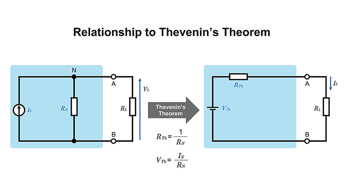
Thevenin’s theorem says that “any two-terminal linear circuit can be reduced to a single voltage source V_Th in series with R_Th.” Norton’s theorem can describe the same circuit with a current source I_N parallel with R_N. The relationship is:

\(I_N=\displaystyle \frac{V_{Th}}{R_{Th}} , R_N=R_{Th}\)

In other words, the information is identical, just expressed differently.

Points for Deciding Which to Use

Both theorems help simplify circuits, but specific scenarios make each more intuitive:

• Thevenin form: Voltage source (V_Th) + series resistor (R_Th)
  • Useful when focusing on voltage or power.
  • Convenient when you want to see how voltage changes as you vary the load.
• Norton form: Current source (I_N) + parallel resistor (R_N)
  • Helpful in analyzing current flow, mainly how it divides among parallel branches.
  • Can simplify tasks involving parallel connections.

Depending on the circuit layout, one form may feel more natural.

Norton’s Theorem in Circuits with Dependent/AC Elements

Real-world or research-level circuits often contain dependent sources and AC components, not independent sources and resistors. Even so, Norton’s theorem can apply as long as linearity holds. Below, we discuss what to watch for when Norton’s theorem is used in circuits that involve dependent sources or frequency-dependent elements.

When Dependent Sources Are Involved

Dependent sources (controlled sources) are voltage or current sources whose values depend on another electrical quantity in the circuit. Norton’s theorem can be used as long as the circuit remains linear overall, but you must keep the dependent sources in place when zeroing out the independent sources.

You cannot entirely remove the dependent source from the circuit; you must keep it to maintain its controlling equation while calculating I_N and R_N.

Frequency‑Dependent Components

If capacitors or inductors are present, the circuit has frequency-dependent impedances. By representing each capacitor or inductor with its complex impedance, you can extend Norton’s theorem to AC analysis of linear circuits.

For instance,

\(Z_C=\displaystyle \frac{1}{jωC} , Z_L=jωL\)

You can then treat the circuit in the complex domain. The resulting Norton equivalent is a current source parallel to a complex impedance R_N. The process for short-circuit current and zeroing out sources is conceptually the same, just done in terms of complex numbers.

Applications for Maximum Power Transfer and Load Adjustment

Norton’s theorem simplifies circuit geometry and helps evaluate power transfer or load current calculations when load conditions change. In particular, the well-known maximum power transfer problem can be solved more intuitively using a Norton equivalent. This section shows how Norton’s form offers insights for optimizing load conditions and computing power.

Condition for Maximum Power Transfer

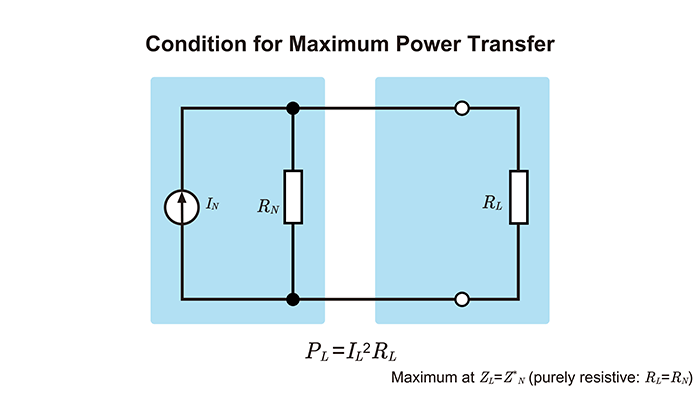
Maximum power is delivered to the load when the load impedance is the complex conjugate of the source (Norton/Thevenin) output impedance:

\(Z_L = Z_N^*\)(equivalently, R_L = R_N and X_L = –X_N ).

In the purely resistive case (DC or when the output impedance is real), this reduces to R_L = R_N.

Using the Norton equivalent may simplify the analysis when choosing or adjusting R_L in a design. One example is in amplifier output stages, where you want the load to match the output impedance for maximum efficiency.

Quickly Evaluating Load Current Changes

Once you know I_N and R_N, you can easily see how the load current changes as R_L varies.

If you have

\(I_L=\displaystyle \frac{I_N×R_N}{R_N+R_L}\)

This is the parallel circuit current split, and the load voltage can be found from

\(V_L =I_L ×R_L\)

You can do these same calculations in Thevenin form, but Norton form is often more straightforward for analyzing current division.

Advanced Topics and Norton’s Theorem

Once you’ve learned Norton’s theorem, you’ll find that combining it with other principles or theorems is vital in practice. Especially in circuits with multiple sources or complex connections, using Millman’s theorem or superposition can help break down problems systematically. This section highlights a few advanced topics closely related to Norton’s theorem to deepen your understanding further.

Relation to Millman’s Theorem

Millman’s theorem finds the combined voltage of multiple voltage sources connected in parallel with internal resistances. Applying Norton’s theorem in many steps, you do the same calculations for current sources in parallel or combine internal resistances. The approach is very similar to what Millman’s theorem formalizes.

Pairing with the Superposition Theorem

As mentioned, calculating the Norton current (I_N) often employs the superposition theorem in circuits with multiple independent sources. You consider each source one at a time, find the short-circuit current, and sum them up. Though it might look repetitive, especially in small circuits, it has a straightforward systematic procedure and works well with Norton’s theorem.

Approximate Analysis of Nonlinear Elements

While this article assumes linear circuits, real semiconductor circuits can include nonlinear devices. Even then, if you linearize the circuit around an operating point, you can use a Norton equivalent for approximate analysis. For example, treat the transistor’s base-emitter junction like a diode, extract its small-signal impedance, represent the collector current as a dependent source, and so on.

Norton’s theorem becomes more challenging to apply to large swings that cross multiple operating regions. In these cases, you would typically switch to simulation or numerical methods.

Conclusion

We have explored the key concepts of Norton’s theorem, how to derive the equivalent circuit, its relationship with Thevenin’s theorem, and applications in more complex situations. Finally, let’s recap the critical points and consider how to use Norton’s approach in future circuit design or study. By mastering the Norton form, you can more clearly determine voltages and currents in circuits with multiple sources and loads.

Norton’s theorem is, alongside Thevenin’s theorem, one of the foundational methods for circuit analysis. Below are the highlights:

• Any two-terminal linear circuit can be expressed as an ideal current source I_N parallel with a resistor R_N.
• I_N is the current that flows when those terminals are short-circuited, and R_N is the two-terminal resistance with all independent sources set to zero.
• Relationship with Thevenin’s theorem:
  • Thevenin voltage V_th = I_N × R_N, and Thevenin resistor R_th = R_N.
• Practical analysis approach:
  • Superposition or node analysis can be used to find I_N and R_N.
• Wide range of applications:
  • Circuits with dependent sources or AC components, maximum power transfer, and load adjustments.