What Is Nodal Analysis (Nodal Voltage Analysis)?

Nodal analysis（Nodal Voltage Analysis, Node Voltage Method） is a circuit analysis method that treats the voltage at each node in a circuit as an unknown and uses Kirchhoff’s Current Law (KCL) to set up a system of simultaneous equations. By applying nodal analysis, even circuits with many resistors and power supplies can be clearly solved for the voltage at each node. For example, nodal analysis is widely used in designing circuits for everyday electronic devices such as smartphones and home appliances. This article explains the detailed calculation procedure of nodal analysis.

Overview of Nodal Analysis

Nodal analysis is a method for analyzing an electrical circuit by defining the electric potential at each node (junction) as an unknown and applying KCL to express the total current flowing into and out each node. As circuits become more complex, tracking every current and voltage individually can be demanding. However, nodal analysis focuses on node-to-node voltage differences, making it efficient to reduce the problem to a set of simultaneous equations.

Nodes and Reference Node

In general, choose any point in the circuit as the reference node (often called ground). This reference node serves as the reference point in the circuit. All other nodes are then defined by their voltage relative to this reference point. Because the total number of unknown voltages is “number of nodes − 1,” nodal analysis reduces the size of the system even when the circuit is large.

Theoretical Basis of Nodal Analysis

Nodal analysis mainly uses Kirchhoff’s Current Law (KCL) in combination with Ohm’s Law. KCL ensures that the net current flowing into a node equals the net current flowing out, and Ohm’s Law provides the linear relationship between voltage and current. By combining these laws, one can write an equation for each node and then solve the resulting system of equations to analyze the entire circuit.

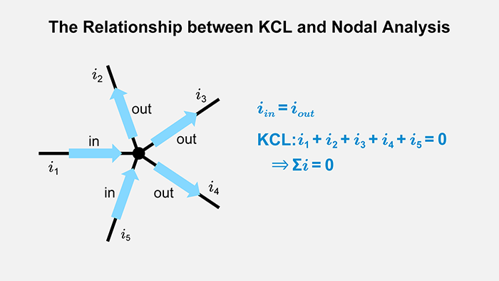
Applying Kirchhoff’s Current Law (KCL)

Focusing on a single node, the sum of currents flowing into the node and the sum of currents flowing out of the node are equal:

\(i_1+i_2+⋯+i_n=0\)

This is the fundamental equation for nodal analysis.

Ohm’s Law and Impedances

Each branch (resistor or impedance) current can be expressed by dividing the potential difference across that element by its resistance or impedance. For a resistor R,

\(i=\displaystyle\frac{V_1-V_2}{R}\)

Similarly, capacitors and inductors can be handled using their frequency-domain impedances jωL and 1/(jωC).

Basic Procedure of Nodal Analysis

Below is an outline of how to apply nodal analysis step by step and some points to remember. Even in large and complex circuits, by following these steps in sequence, you can efficiently solve for the unknown node voltages. In addition, this section includes details on using matrix form (the matrix method) for the computations, including intermediate steps.

Step 1 – Selecting the Reference Node

Pick one node in the circuit to be the reference node (ground) at 0V. It’s common to choose the node that connects to the most components or the node used as the circuit’s ground terminal to reduce the number of unknowns and simplify the calculations.

Points to Note about Choosing a Reference Node

• A node with many connected components (resistors, power supplies, loads, etc.) is generally chosen to simplify the equations’ setup.
• In circuits with multiple power supplies or mixed DC and AC sources, which node to choose may not be immediately apparent. However, picking the node that simplifies post-calculation tasks is often advantageous.

Step 2 – Defining the Node Voltages

Assign a voltage V₁, V₂, …, V_n to each node except for the reference node. If there are N total nodes, there will be (N −1) unknowns. This systematic approach clarifies how many variables you need, even in large circuits.

Step 3 – Writing KCL Equations for Each Node

For each node,

\(Σ(incoming current)=0\)

Use Ohm’s Law to express the current flowing through each connected resistor or impedance.

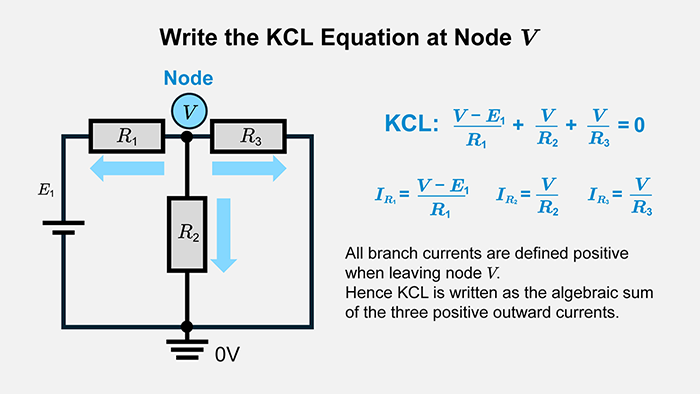
• Example: When node V is connected to the voltage source node E₁ through resistor R₁ and, additionally, to the reference node G = 0V through resistors R₂ and R₃, the KCL at node V is

  \(\displaystyle\frac{V-E_1}{R_1}+\displaystyle\frac{V}{R_2}+\displaystyle\frac{V}{R_3}=0\)

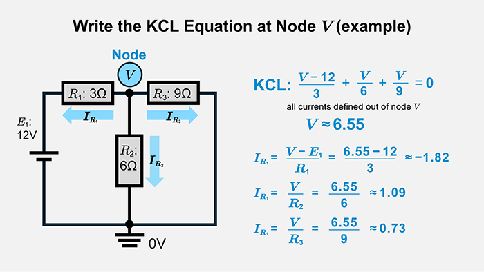
Detailed Example of Intermediate Calculations

Given R₁=3Ω, R₂=6Ω, R₃=9Ω, a voltage source E₁=12V, and an unknown node voltage V, the KCL at node V is

\(\displaystyle\frac{V-12}{3}+\displaystyle\frac{V}{6}+\displaystyle\frac{V}{9}=0\)

\(⟹V≈6.55V\)

The equation derived from KCL is also called a node equation (node-voltage equation).
If additional nodes exist, write similar equations for each one and solve the resulting simultaneous system to obtain every node voltage.

Step 4 – Arranging into Matrix Form and Solving

Once you have the set of simultaneous equations, arranging them in matrix form allows a more systematic approach. Linear algebra methods can handle large-scale circuits. A computer-based matrix solver is typically used when the unknown count is high.

• General Matrix Form: GV =I, where x is the vector of unknown node voltages, G is the coefficient matrix derived from the circuit’s resistors and connections, and I is the vector of constant terms (due to sources). If G is constructed correctly, then V = G⁻¹I.

This representation can also be called a matrix equation, highlighting the problem’s linear algebraic nature.

An Example of the Matrix Method

If you decide to include node voltages and certain currents as unknowns, you can represent them together in a matrix. The approach depends on the number of resistors and power sources you have.

1. Convert the KCL, voltage source constraints, etc., into matrix form.
2. Solve GV = I using inverse matrices or Gaussian elimination.

By writing down the intermediate steps, you can check your calculations more reliably and see precisely how each current and voltage fits into the system.

Note: In planar circuits with many voltage sources but only a few loops, mesh analysis can yield fewer unknowns (see the companion article for details).

Dealing with Supernodes

If an independent voltage source is connected directly between two non-reference nodes, a basic KCL approach at those nodes alone is not enough. This case is called a supernode, and you need an additional voltage constraint equation.

Below is a look at how to integrate supernodes into nodal analysis and express them in matrix form.

The Concept of a Supernode

A supernode is formed when a voltage source connects two nodes. You treat these two nodes as one combined node from a KCL perspective, but you must also include the condition V₁ – V₂ = voltage source.

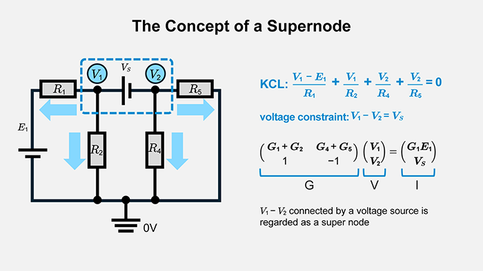
Polarity Concerns with Voltage Sources

• Getting the polarity reversed—whether V₁ –V₂= V_S or V₂ – V₁ = V_S —leads to sign errors and incorrect results.

Supernode Equations and Intermediate Calculations

For example, if nodes A and B are connected by an independent voltage source V_S, and each node has a resistor to the reference node, the supernode is A plus B combined. Then:

1. KCL (the entire supernode)

   (V₁−0)/R₁+(V₂−0)/R₂+…=0

2. Voltage Source Constraint

   V₁−V₂=V_S

These equations are then included in your overall system. The KCL for the supernode is one equation, and the voltage source constraint is another. Both go into GV = I.

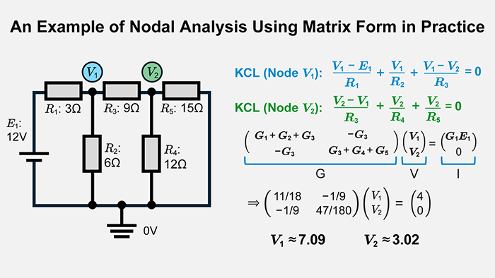
An Example of Nodal Analysis in Practice

Here, we present a simplified circuit example with numerical values to illustrate how to apply nodal analysis step by step. This is more comprehensive than the smaller examples mentioned earlier. It also shows how to simultaneously treat certain currents and node voltages within a matrix solution, without skipping intermediate steps.

Problem Setup

For the circuit below—which contains multiple voltage sources and resistors—determine the node voltages V₁, V₂ and branch currents I₁, I₃.

• Voltage source (with respect to the reference node 0V)

  E₁=12V

• Resistors

  R₁=3Ω, R₂=6Ω, R₃=9Ω, R₄=12Ω, R₅=15Ω

Concrete Example — Choice of Unknowns

• Node voltage V₁, V₂
• Branch currents I₁, I₃

Forming the Simultaneous Equations

1. KCL at Node V₁

   \(\displaystyle\frac{V_1-E_1}{R_1}+\displaystyle\frac{V_1}{R_2}+\displaystyle\frac{V_1-V_2}{R_3}=0\)

2. KCL at Node V₂

   \(\displaystyle\frac{V_2-V_1}{R_3}+\displaystyle\frac{V_2}{R_4}+\displaystyle\frac{V_2}{R_5} =0\)

   Express each resistor as a conductance,

   \(G=\begin{pmatrix} G_1+G_2+G_3 & -G_3 \\ -G_3 & G_3+G_4+G_5 \end{pmatrix}, V=\begin{pmatrix} V_1 \\ V_2 \end{pmatrix}, I=\begin{pmatrix} G_1 E_1 \\ 0 \end{pmatrix}\)

Substituting Numbers and Calculating

Substituting Numbers

\(G=\begin{pmatrix} \displaystyle\frac{11}{18} -\displaystyle\frac{1}{9} \\ -\displaystyle\frac{1}{9} \displaystyle\frac{47}{180} \end{pmatrix}, I=\begin{pmatrix} 4 \\ 0 \end{pmatrix}\)

\(V=G^{-1} I ⟹ V_1≈7.09 [V],V_2≈3.02 [V]\)

Calculating Branch Currents

\(I_1=\displaystyle\frac{E_1-V_1}{R_1} ≈1.64 [A],I_3=\displaystyle\frac{V_1-V_2}{R_3} ≈0.45 [A]\)

Extending Nodal Analysis to AC Circuits and Frequency Domain

Nodal analysis can handle both DC and AC circuits. In AC analysis, it is necessary to account for the frequency-dependent behavior of inductors and capacitors. However, we can set up the nodal equations like we do for DC using impedances Z.

In a DC analysis, resistors are simply R. In the frequency domain, each component’s impedance is:

• Inductor L：Z_L = jωL
• Capacitor C：Z_C = 1/(jωC)
• Resistor R：Z_R = R

Phasors and Complex-Number Analysis

When sinusoidal sources drive the circuit, each node voltage can be expressed as a phasor (a complex number representing magnitude and phase). Applying nodal analysis similarly, each KCL equation uses complex impedances instead of real resistances. For a node voltage V and a neighboring node voltage V_X with an impedance Z between them: i= (V – V_X)/Z.

Z may be real (resistive) or complex (inductive or capacitive). The final result is a set of complex-valued node voltages.

Matrix Form in the Frequency Domain

As in the DC case, you gather each KCL equation into a matrix form, but now the matrix elements are complex numbers. The steps are:

1. Define the nodes and pick a reference node
2. Identify each resistor, inductor, and capacitor
3. Write KCL in terms of complex impedances: (V₁–V₂)/Z₁₂+(V₁–V₃)/Z₁₃+… = 0
4. Convert to matrix form: Y(ω)V = I(ω)
5. Solve for V using complex linear algebra

One can plot frequency responses, such as Bode plots, by repeating the calculation for various frequencies.

Extension of Node Analysis to Dependent Sources, Nonlinear and Large-scale Circuits

Handling the Four Types of Dependent Sources

There are four kinds of dependent (controlled) sources: the Voltage-Controlled Voltage Source (VCVS), the Current-Controlled Voltage Source (CCVS), the Voltage-Controlled Current Source (VCCS), and the Current-Controlled Current Source (CCCS). In every case, the source’s output is determined by a voltage or current measured at another point in the circuit.

• VCVS, CCVS: add an extra voltage constraint row to the matrix. (CCVS uses the control current I_X as the new variable.)
• VCCS, CCCS: add the coefficient to the corresponding admittance entry. (VCCS: g_m, CCCS: k)

Linearization and Iterative Methods

Many practical circuits include nonlinear elements like diodes, transistors, or MOSFETs. Even in such cases, nodal analysis can be the foundation for a numerical approach.

Voltage-current relationships are no longer strictly proportional when a circuit contains nonlinear devices. In such situations, the circuit can be linearized around an operating point, and iterative approaches (such as Newton-Raphson) are used. Tools like SPICE implement these methods under the hood.

Approximation of Nonlinear Elements and Operating Point Analysis

• Diodes, BJTs, MOSFETs, etc., have exponential or otherwise nonlinear I-V characteristics.
• Although nodal analysis is still the overarching framework, nonlinear devices make the system of equations nonlinear, so standard matrix inversion is insufficient.
• The basic approach is to approximate the device behavior around an operating point with a small-signal equivalent (the derivative-based slope), solve the resulting linear system, and then update the estimates until the solution converges.

Nodal Analysis in Circuit Simulation

Most circuit simulators (such as those in the SPICE family) rely on nodal analysis internally. While the user only sees a schematic editor, the software numbers each node, treats them as unknown voltages, and solves KCL-based equations.

SPICE Fundamentals and Nodal Analysis

SPICE includes many device models and electromagnetic coupling elements, but the core is still a nodal analysis approach. In the presence of nonlinear elements, SPICE repeatedly adjusts the operating point using iterative solvers until the node voltages and currents stabilize.

Benefits of Semiconductor Circuit Design

Nodal analysis is suitable for large-scale circuits because it follows the same steps regardless of circuit size. IC design and semiconductor processes often rely on nodal analysis. Although the number of nodes grows, the essential method remains the same.

A semiconductor chip contains numerous transistors, resistors, and parasitic elements, leading to many nodes. By formulating nodal equations as a matrix and using numerical solvers, one can determine the node voltages for the entire circuit.

Comparison with Mesh Analysis

Another principal circuit analysis method is mesh analysis, which uses Kirchhoff’s Voltage Law (KVL) to define unknown loop currents. Whether to use nodal (KCL-based) or mesh (KVL-based) analysis depends on the circuit’s shape and the presence of certain elements.

Application Ranges and Choosing the Right Method

• Mesh analysis may have fewer unknowns for planar circuits with a few loops.
• Circuits with many voltage sources or nonplanar structures often favor nodal analysis, especially when it’s more natural to think about voltages than loop currents.
• When circuits become large, nodal analysis is more scalable, especially for computer implementations.

A hybrid analysis approach is also practical for small circuits solved by hand. In this hybrid approach, the loop currents are first directly determined using the mesh method (KVL), and then these results are used to back-calculate the node voltages with nodal analysis. By first determining the currents, it becomes easier to handle voltage sources and shared resistors that can be challenging with nodal analysis alone. This makes it simpler to maintain consistency and accuracy when solving circuits by hand.

Conclusion

Nodal analysis is a powerful, systematic way to handle circuit analysis. Treating each node voltage as an unknown allows one to represent even large circuits as a set of simultaneous equations. This applies to resistive circuits, AC analysis (using complex impedance), and nonlinear circuits (through linearization and iterative methods). Nodal analysis also manages exceptional cases such as supernodes—where two non-reference nodes are directly connected by a voltage source—by adding an extra constraint equation. SPICE and similar simulation tools are built on these principles, making nodal analysis pervasive in modern electronic circuit design. With a solid understanding of nodal analysis, one can confidently tackle increasingly large and complex circuits.