Learn Know-how

Basics of Spectrum

2018.01.11

Points of this article

・As the frequency is raised, the overall spectrum amplitude increases.

・When rise/fall times are slowed (increased), the frequency from which -40dB/dec attenuation begins is lower, and the spectrum amplitude is attenuated.

・When the duty cycle is changed, even-numbered harmonics appear, but there is no effect on the spectrum peak. The fundamental wave spectrum is attenuated.

・When only the rise time is slowed, tr components are attenuated from a lower frequency.

table of contents

・The Basics of Spectrum
・Waveform Changes and Changes in the Spectrum

Previously, as basic knowledge of EMC, the meanings of various terms related to EMC were explained in the section titled “What is EMC?”. This time, we shall explain the basics of a spectrum.

In reviewing basic knowledge, we begin by briefly considering the question “what is a spectrum?” According to the Concise Electronics Dictionary Edition of the Encyclopedia Britannica, a spectrum is “the result of analyzing an electromagnetic wave into its sine wave components and arranging the components in order of wavelength”, and by extension means “analyzing something with a complex makeup into simple components, and arranging the components in order of the magnitude of a characterizing quantity…”. This is a comparatively matter-of-fact explanation, but upon considering it carefully, we can see that it is reasonable.

The spectra we will be considering here are the spectra of electrical signals. More specifically, we will be explaining spectra using data obtained using a spectrum analyzer that plots frequency along the horizontal axis, and power or voltage along the vertical axis.

The Basics of Spectrum

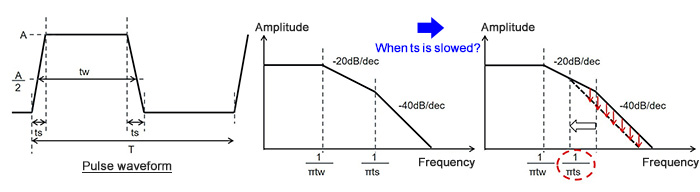
We begin with the following schematic diagrams. Here the topic is “EMC of a switching power supply”, and so it is assumed that an electrical signal is a switching signal. We begin our explanation using the diagrams below, in which a switching signal, represented as a pulse waveform, is characterized by tw (the pulse width) and ts (the rise time/fall time).

The graph in the center represents the spectrum of theoretical pulse waveforms obtained from a Fourier transform. This is a familiar spectrum in which, as the frequency rises, the amplitude attenuates, and the slope of the attenuation changes with tw and ts.

The graph on the right shows the change in the spectrum when the pulse ts is made slower (increased). It is natural that when the slope changes to -40 dB/dec the frequency at 1/πts is lower, but as a result, the subsequent amplitude is reduced. Put simply, when ts is slowed, the spectrum amplitude is attenuated.

EMC_2_graf01

From here, we shall use actual spectrum analyzer data to observe changes in a spectrum with changes in the frequency and other parameters. What should be noted here is the manner in which the spectrum tends to change with changes in the signal waveform. This knowledge will be necessary when analyzing EMC and devising countermeasures using spectra related to the switching of an actual switching power supply circuit.

Waveform Changes and Changes in the Spectrum

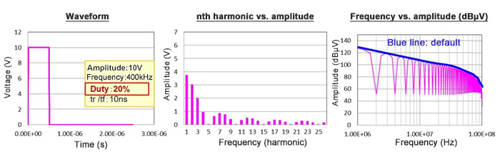
The first graph shown below presents the default conditions, to be used as a basis for comparison. As indicated in the waveform graph, these conditions are an amplitude of 10 V, a frequency of 400 kHz, a duty cycle of 50%, and a tr/tf (rise time/fall time) of 10 ns.

The center graph shows nth harmonics and amplitudes (V). The amplitude is greatest for the first harmonic which is the fundamental wave, that is, the 400 kHz component, and the spectrum appears at the frequencies of the odd-numbered harmonics.

EMC_2_graf02

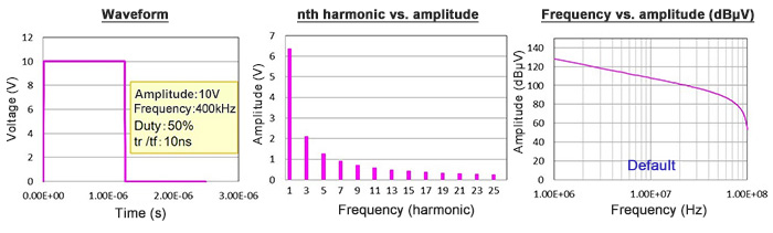
The presence of only odd-numbered harmonics is a characteristic of a spectrum with a duty cycle of 50% = 1:1. The magnitude of each component is the reciprocal of the harmonic number times the fundamental wave component, so that, for example, the magnitude of the third harmonic is 1/3 of the fundamental wave amplitude, and the nth harmonic is 1/n of the amplitude.

The graph on the right is a logarithmic plot of the amplitude, as dBμV. Here dBμV is the decibel value of the voltage ratio with a 1 μV voltage as reference.

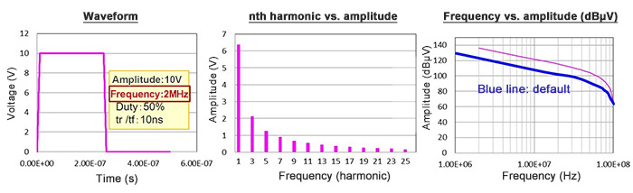
①In the spectrum below, the frequency is changed to 2 MHz. As is clear from the frequency vs. amplitude (dBμV) graph, when the frequency is higher, the overall amplitude is increased.

EMC_2_graf03

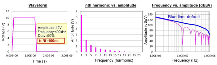
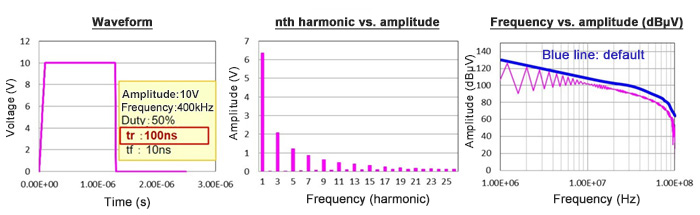
②And in the spectrum below, both tr and tf are slowed (increased) to 100 ns. As explained using the schematic diagrams above, the frequency at which the -40 dB/dec attenuation begins is lowered, and the spectrum amplitude is attenuated.

EMC_2_graf04

③This is a spectrum in which the duty cycle is reduced from 50% to 20%. The duty cycle is no longer 1:1, and so even-numbered harmonics appear, but in essence there is no change in the peak. By narrowing the pulse width tw, the amplitude of the fundamental wave spectrum is attenuated.

EMC_2_graf05

④The spectrum below is a case in which only tr (the rise time) is slowed. Components related to tr are attenuated from lower frequencies due to the slower tr.

EMC_2_graf06

The respective results are listed. To summarize, when the frequency is low and the rise/fall times are slow, the spectrum is attenuated. From the standpoint of EMC, put simply, a lower spectrum amplitude is advantageous.

①Raising the frequency
②Slowing the rise/fall times
③Changing the duty cycle
④Slowing only the rise time

⇒ Overall increase in spectrum amplitude
⇒ Lower frequency from which -40dB/dec attenuation begins,
attenuation of spectrum amplitude
⇒ Appearance of even harmonics, but no effect on spectrum peak.
Attenuation of the fundamental wave spectrum
⇒ tr components attenuated from lower frequency

In the next section, we will discuss differential mode and common mode noise.

【Download Documents】 Elementary EMC for Circuit Designers Working on EMC Issues

This handbook is designed to give designers who are going to work on EMC an idea of what EMC is. It promotes a sensible understanding of the relationship between EMC and the three perspectives of semiconductor devices, product specifications, and circuits and boards.

Download

Learn Know-how

Electrical Circuit Design

Thermal design

Switching Noise

Simulation